Install IPython libraries (If necessary)

pip install ipython

pip install ipykernel

pip install ipywidgets

Import scEGOT class and other libraries. We use copy, os, itertools, anndata, Ipython.display.display and pandas to read and reshape input data.

import copy
import itertools
import os

import anndata
from IPython.display import display
import pandas as pd

from scegot import scEGOT

Set constants

DATASET_INPUT_ROOT_PATH = os.path.join(os.getcwd(), "dataset/")
RANDOM_STATE = 2023
PCA_N_COMPONENTS = 30
GMM_CLUSTER_NUMBERS = [1, 2, 4, 5, 5]
UMAP_N_NEIGHBORS = 1000
DAY_NAMES = ["day0", "day0.5", "day1", "day1.5", "day2"]

In case of Anndata :

ANNDATA_FILE_NAME = 'GSE241287_scRNAseq_hPGCLC_induction'
ANNDATA_DATASET_PATH = os.path.join(DATASET_INPUT_ROOT_PATH, ANNDATA_FILE_NAME) + '.h5ad'

In case of DataFrame(CSV) :

DATAFRAME_FOLDER_NAME = 'GSE241287_RAW'
DATAFRAME_DATASET_FOLDER_PATH = os.path.join(DATASET_INPUT_ROOT_PATH, DATAFRAME_FOLDER_NAME)

Read input files

Either AnnData or DataFrame (CSV) can be used.

• In the case of AnnData: The name of the obs key containing the day information is passed as the adata_day_key argument when instantiating the scEGOT class.

• In the case of DataFrame: One DataFrame must correspond to each day; prepare an array of DataFrames in the order of day.

The following scRNA-seq data of the human PGCLC induction system are available in the Gene Expression Omnibus GEO under identification number GSE241287.

The data is expected to be stored in ./scegot/dataset, DATASET_INPUT_ROOT_PATH.

In case of Anndata :

input_data = anndata.read_h5ad(ANNDATA_DATASET_PATH)
print(input_data)
display(input_data.X)
display(input_data.obs)
display(input_data.var)

AnnData object with n_obs × n_vars = 11771 × 18922
    obs: 'sample', 'percent.mito', 'day', 'cluster_day'
    var: 'spliced', 'unspliced', 'mt', 'TF', 'gene_name'
    layers: 'X_raw', 'spliced', 'unspliced'

<Compressed Sparse Row sparse matrix of dtype 'float32'
        with 94477374 stored elements and shape (11771, 18922)>

	sample	percent.mito	day	cluster_day
iM.data_GTGGAAGGTCAATGGG-1	iM.data	0.056487	iM	day0
iM.data_TTCATGTCAACCCGCA-1	iM.data	0.216231	iM	day0
iM.data_GAGGGTATCCAGGACC-1	iM.data	0.076525	iM	day0
iM.data_AAGTCGTAGGCTTTCA-1	iM.data	0.080264	iM	day0
iM.data_ACCGTTCGTAACTTCG-1	iM.data	0.280788	iM	day0
...	...	...	...	...
d2b.data_AAGCCATAGGGCGAGA-1	d2b.data	4.811476	d2b	day2
d2b.data_CAACCAATCTTCCGTG-1	d2b.data	2.554428	d2b	day2
d2b.data_AGGCCACGTGAGTAGC-1	d2b.data	3.142146	d2b	day2
d2b.data_GATCAGTTCGAGTACT-1	d2b.data	4.287140	d2b	day2
d2b.data_TCATCCGTCATGGGAG-1	d2b.data	2.835834	d2b	day2

11771 rows × 4 columns

	spliced	unspliced	mt	TF	gene_name
FAM3A	1	1	0	0	FAM3A
SLC25A1	1	1	0	0	SLC25A1
RBL1	1	1	0	0	RBL1
PPP2R1A	1	1	0	0	PPP2R1A
H3F3B	1	1	0	0	H3F3B
...	...	...	...	...	...
OR2W5	1	0	0	0	OR2W5
ODF4	1	1	0	0	ODF4
CRP	1	0	0	0	CRP
KRTAP4-9	1	0	0	0	KRTAP4-9
THEMIS	1	1	0	0	THEMIS

18922 rows × 5 columns

In case of DataFrame(CSV) :

input_file_paths = [f"{DATAFRAME_DATASET_FOLDER_PATH}/{day_name}.csv" for day_name in DAY_NAMES]
input_data = [
    pd.read_csv(input_file_path, index_col=0).T for input_file_path in input_file_paths
]

print("shape of each day's data:")
for i, data in enumerate(input_data):
    print(f"    {DAY_NAMES[i]}: {data.shape}")
print("data example: ")
input_data[0].head()

tf_gene_names = (
    pd.read_csv(
        f"{DATASET_INPUT_ROOT_PATH}/TFgenes_name.csv", header=None
    )
    .values[0]
)
tf_gene_names

array(['cell', 'ZBTB8B', 'GSX2', ..., 'NME2', 'ZNF488', 'ZNF280B'],
      dtype=object)

Tutorial

Create scEGOT instance.

You must pass values for the adata_day_key argument when using AnnData and for the day_names argument when using an array of DataFrames. adata_day_key is the key of the day in AnnData.obs, and day_names is an array containing the names of the days in each DataFrames.

In case of Anndata :

scegot = scEGOT(
    input_data,
    verbose=True,  # default=True
    adata_day_key="cluster_day",
)

Processing AnnData...

In case of DataFrame(CSV) :

scegot = scEGOT(
    input_data,
    verbose=True,  # default=True
    day_names=DAY_NAMES, # uncomment this line if you use an array of DataFrames
)

Preprocess:

Preprocess in the following order.

RECODE -> UMI normalize -> log1p normalize -> select variable genes -> PCA

You can also apply UMAP by calling apply_umap() after preprocess(). In the tutorial, UMAP is applied after GMM is applied.

%%time
X, pca_model = scegot.preprocess(
    PCA_N_COMPONENTS,
    recode_params={},
    umi_target_sum=1e5,
    pca_random_state=RANDOM_STATE,
    pca_other_params={},
    apply_recode=True,
    apply_normalization_log1p=True,
    apply_normalization_umi=True,
    select_genes=True,
    n_select_genes=2000,
)

Applying RECODE...
start RECODE for scRNA-seq data
end RECODE for scRNA-seq
log: {'seq_target': 'RNA', '#significant genes': 15820, '#non-significant genes': 2582, '#silent genes': 65, 'ell': 288, 'Elapsed time': '0h 0m 26s 401ms', 'solver': 'randomized', '#train_data': 2354}
Applying UMI normalization...
Applying log1p normalization...
Applying PCA...
        sum of explained_variance_ratio = 83.37207519094473
CPU times: user 5min 5s, sys: 2min 12s, total: 7min 17s
Wall time: 39.6 s

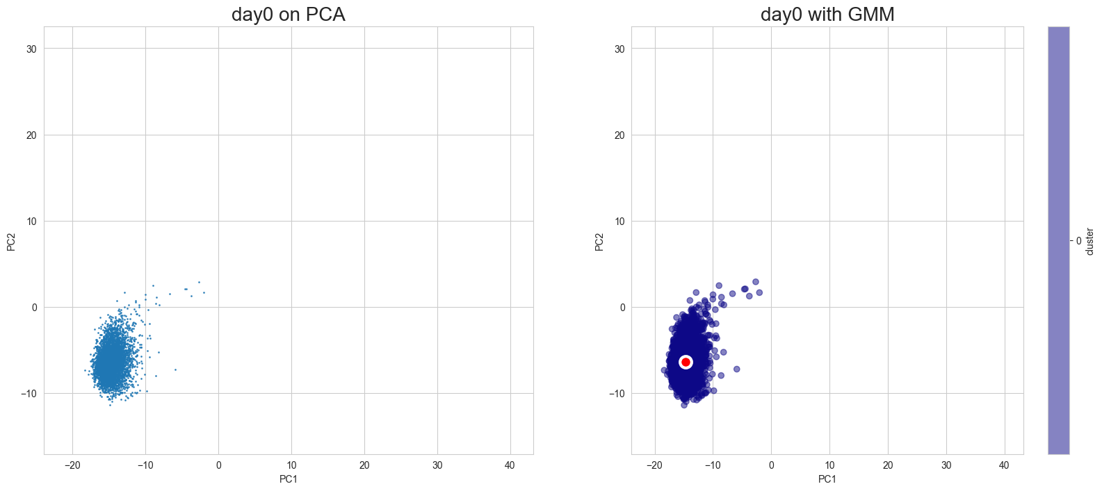
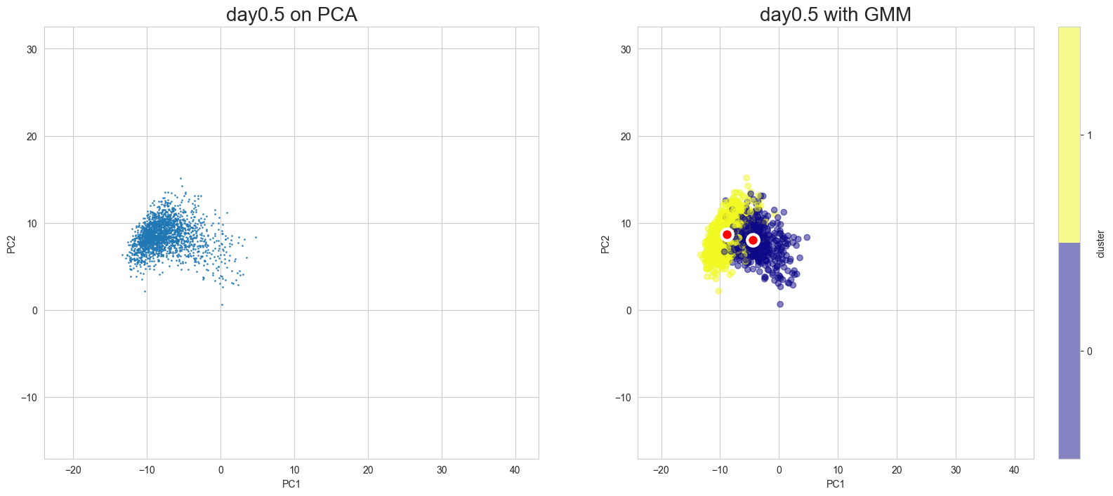
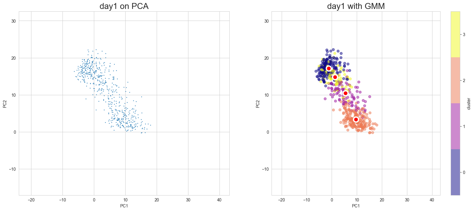
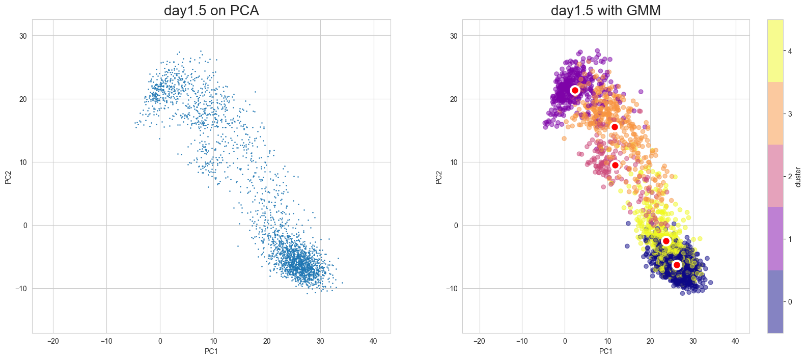
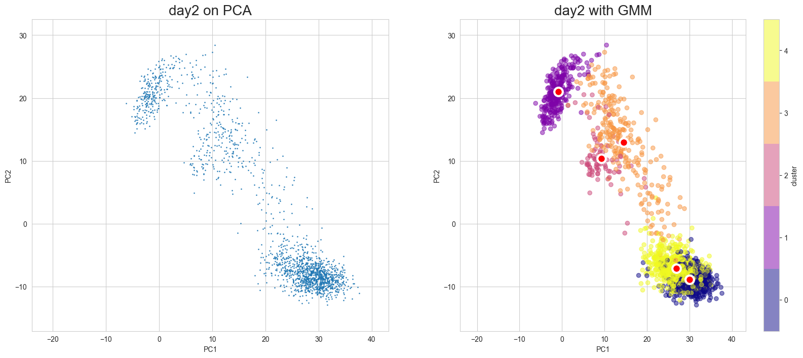
Apply GMM:

Apply GMM and visualize the results in each case of PCA and UMAP. To switch between PCA and UMAP displays, specify the mode argument to the plotting function.

%%time
gmm_models, gmm_labels = scegot.fit_predict_gmm(
    n_components_list=GMM_CLUSTER_NUMBERS,
    covariance_type="full",
    max_iter=2000,
    n_init=10,
    random_state=RANDOM_STATE,
    gmm_other_params={},
)

Fitting GMM models with each day's data and predicting labels for them...

100%|██████████| 5/5 [00:08<00:00,  1.76s/it]

CPU times: user 5min 55s, sys: 7min 34s, total: 13min 30s
Wall time: 8.81 s

Visualization in PCA

scegot.plot_gmm_predictions(
    mode="pca",
    plot_gmm_means=True,
    figure_titles_without_gmm=[f"{name} on PCA" for name in DAY_NAMES],
    figure_titles_with_gmm=[f"{name} with GMM" for name in DAY_NAMES],
    cmap="plasma",
    # save=True,
    # save_paths=[f"./gmm_preds_{day_name}.png" for day_name in DAY_NAMES]
)

Apply UMAP

%%time
X_umap, umap_model = scegot.apply_umap(
    UMAP_N_NEIGHBORS,
    n_components=2,
    random_state=RANDOM_STATE,
    min_dist=0.8,
    umap_other_params={},
)

CPU times: user 3min, sys: 3.46 s, total: 3min 3s
Wall time: 2min

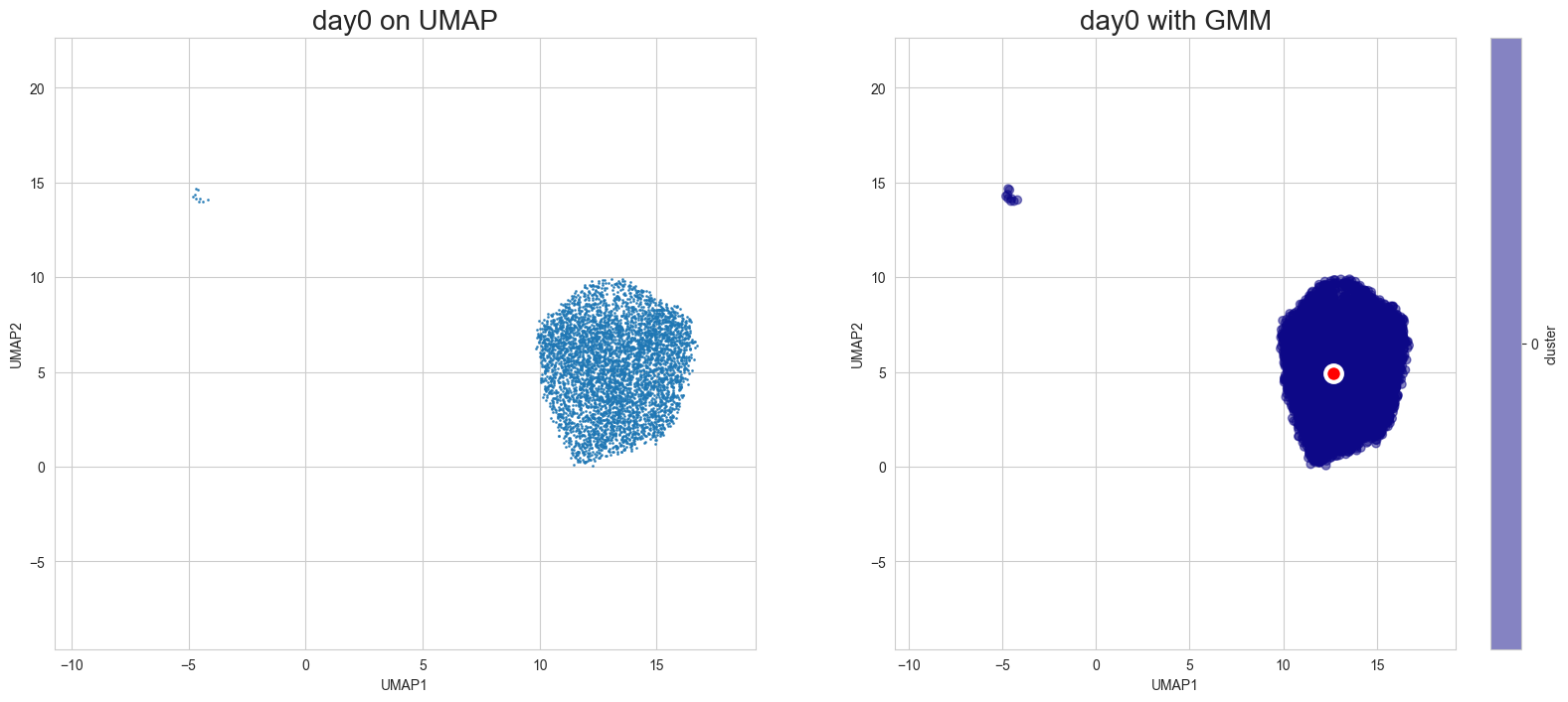
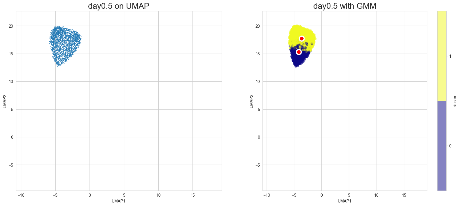
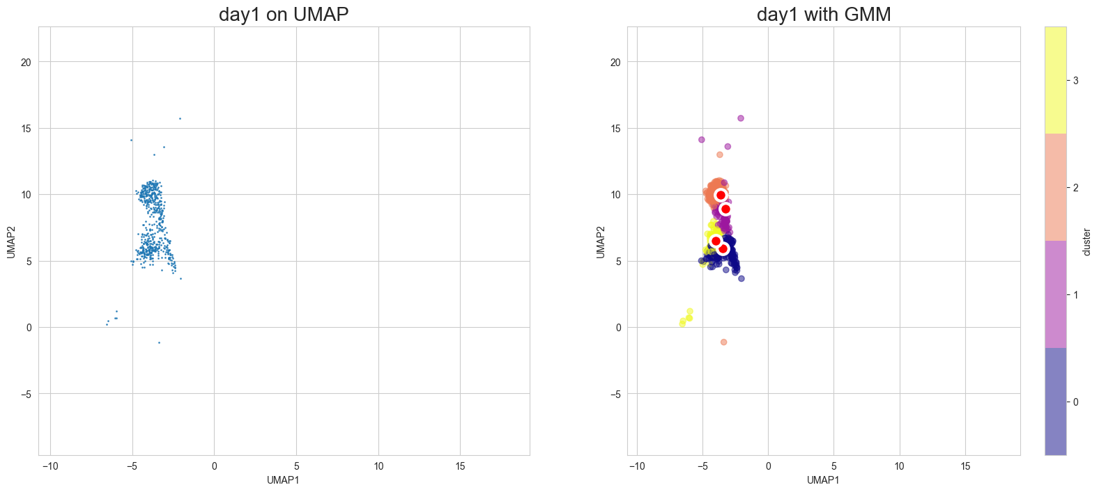
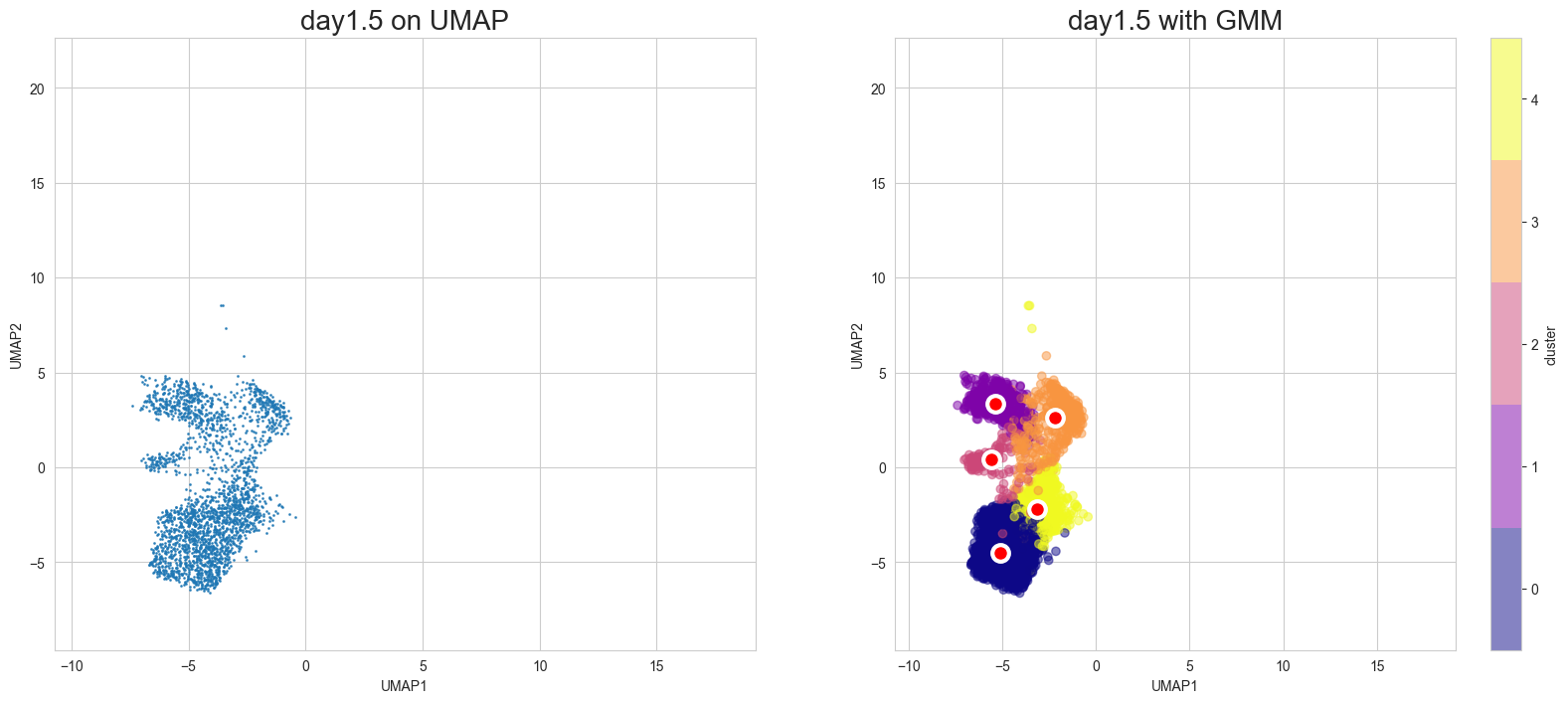
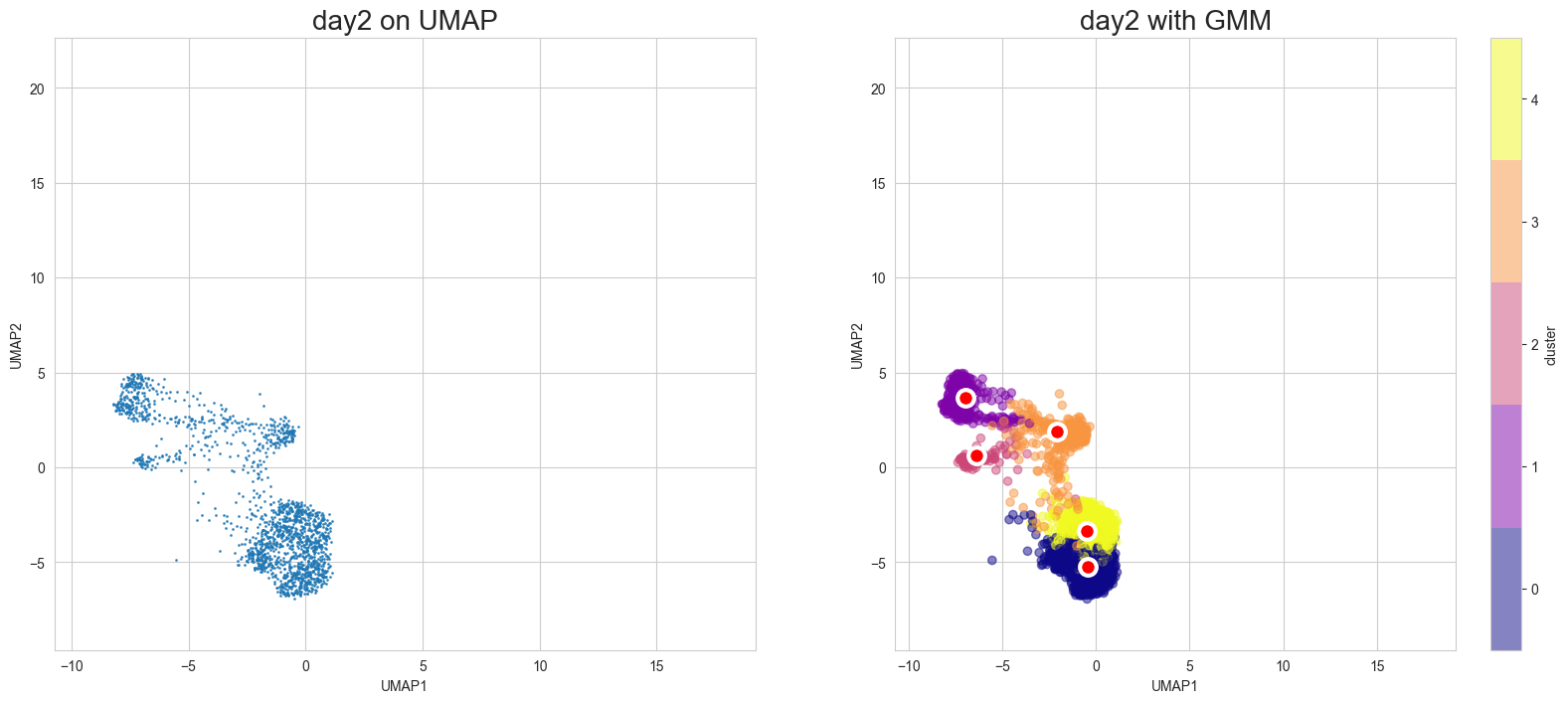
Visualization in UMAP

scegot.plot_gmm_predictions(
    mode="umap",
    plot_gmm_means=True,
    figure_titles_without_gmm=[f"{name} on UMAP" for name in DAY_NAMES],
    figure_titles_with_gmm=[f"{name} with GMM" for name in DAY_NAMES],
    cmap="plasma",
    # save=True,
    # save_paths=[f"./gmm_preds_{day_name}.png" for day_name in DAY_NAMES]
)

Animation of interpolated distribution:

scegot.animatie_interpolated_distribution(
    cmap="gnuplot2",
    interpolate_interval=11,
    # save=True,
    # save_path="./cell_state_video.gif",
)

Interpolating between day0 and day0.5...

100%|██████████| 11/11 [00:03<00:00,  3.25it/s]

Interpolating between day0.5 and day1...

100%|██████████| 10/10 [00:05<00:00,  1.96it/s]

Interpolating between day1 and day1.5...

100%|██████████| 10/10 [00:08<00:00,  1.14it/s]

Interpolating between day1.5 and day2...

100%|██████████| 10/10 [00:10<00:00,  1.04s/it]

Creating animation...

Once Loop Reflect

Cell State Graph:

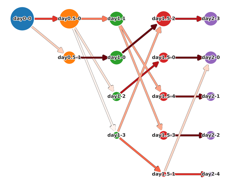
There are two functions for visualizing cell state graphs, one is plot_cell_state_graph() and the other is plot_simple_cell_state_graph(). Both can visualize PCA and UMAP.

Before plotting the graph, call make_cell_state_graph_object() to create a CellStateGraph object. At that time, you can specify cluster names as an array. If not specified, cluster names are automatically generated by the generate_cluster_names_with_day().

There will be other occasions where cluster names are passed in the pathway and cell velocity sections, but it is not necessary for the cluster names in those cases to match the cluster names used in this section. Therefore, the cluster name can be changed flexibly.

cluster_names = scegot.generate_cluster_names_with_day()
cluster_names

[['day0-0'],
 ['day0.5-0', 'day0.5-1'],
 ['day1-0', 'day1-1', 'day1-2', 'day1-3'],
 ['day1.5-0', 'day1.5-1', 'day1.5-2', 'day1.5-3', 'day1.5-4'],
 ['day2-0', 'day2-1', 'day2-2', 'day2-3', 'day2-4']]

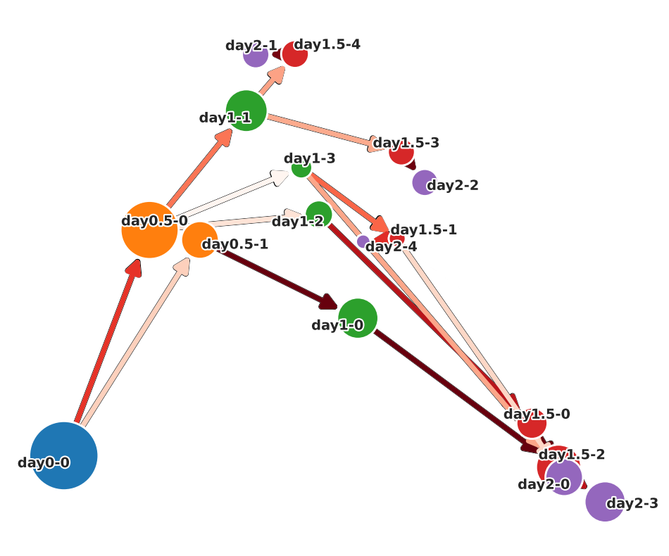
In the case of plot_cell_state_graph()

Weights, gene information and GMM cluster number is displayed in hover texts of the graph.

The shape of the graph can be changed by changing the layout argument.

PCA ver.

csg = scegot.make_cell_state_graph_object(
    cluster_names=cluster_names,
    mode="pca",
    threshold=0.2,
    merge_clusters_by_name=False,
    x_reverse=False,
    y_reverse=False,
    require_parent=True,
)

csg.plot_cell_state_graph_object(
    layout="normal",
    cluster_names=cluster_names,
    tf_gene_names=tf_gene_names,
    tf_gene_pick_num=5,
    # save=True,
    # save_path="./cell_state_graph_pca.png"
)

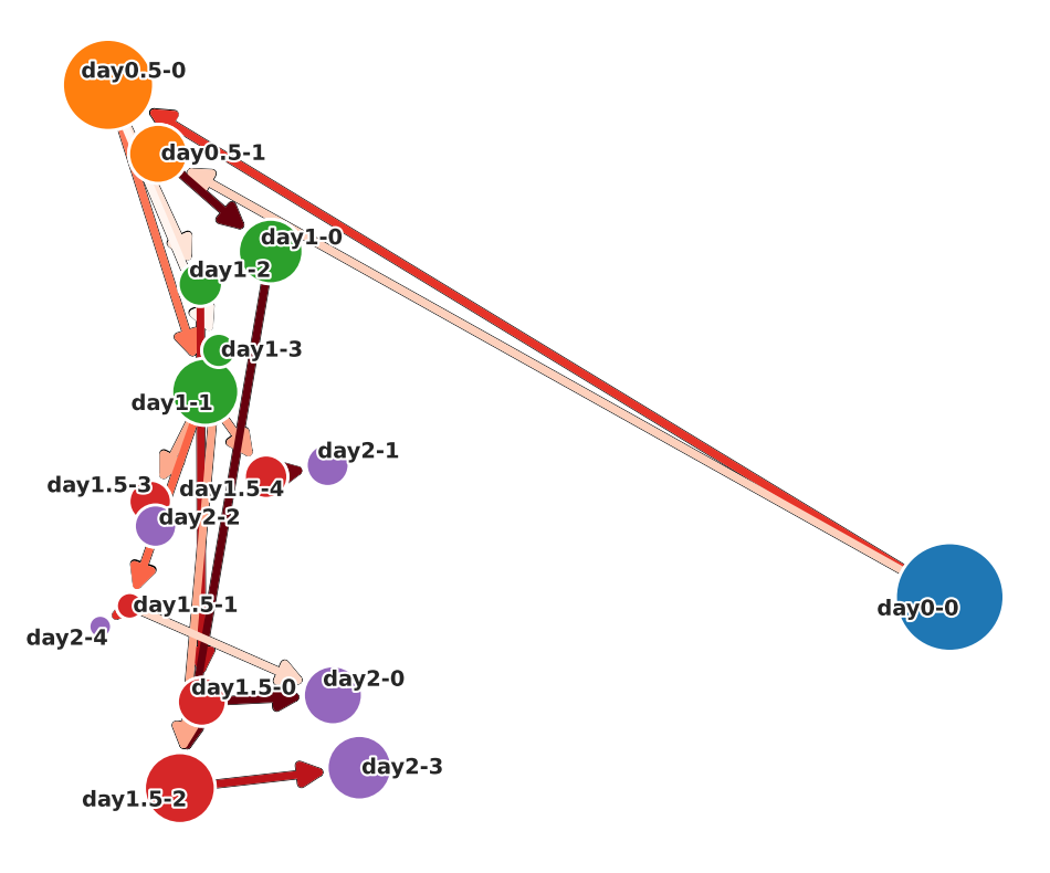
UMAP ver.

csg_umap = scegot.make_cell_state_graph_object(
    cluster_names=cluster_names,
    mode="umap",
    threshold=0.2,
    merge_clusters_by_name=False,
    x_reverse=False,
    y_reverse=False,
    require_parent=True,
)

csg_umap.plot_cell_state_graph(
    layout="normal",
    cluster_names=cluster_names,
    tf_gene_names=tf_gene_names,
    tf_gene_pick_num=5,
    # save=True,
    # save_path="./cell_state_graph_umap.png"
)

layout=”hierarchy”

y_position_dict = {
    "day0-0": 0,
    "day0.5-0": 1, "day0.5-1": 0,
    "day1-0": 0, "day1-1": 2, "day1-2": 1, "day1-3": 3,
    "day1.5-0": 1, "day1.5-1": 4, "day1.5-2": 0, "day1.5-3": 3, "day1.5-4": 2,
    "day2-0": 1, "day2-1": 2, "day2-2": 3, "day2-3": 0, "day2-4": 4
}

csg.plot_cell_state_graph(
    layout="hierarchy",
    y_position=y_position_dict,
    cluster_names=cluster_names,
    tf_gene_names=tf_gene_names,
    tf_gene_pick_num=5,
    # save=True,
    # save_path="./cell_state_graph_hierarchy.png"
)

In the case of plot_simple_cell_state_graph()

You can choose whether to display weights on the graph with arguments.

PCA ver.

csg.plot_simple_cell_state_graph(
    layout="normal",
    cluster_names=cluster_names,
    node_weight_annotation=False,
    edge_weight_annotation=False,
    # save=True,
    # save_path="./simple_cell_state_graph_pca.png"
)

UMAP ver.

csg_umap.plot_simple_cell_state_graph(
    layout="normal",
    cluster_names=cluster_names,
    node_weight_annotation=False,
    edge_weight_annotation=False,
    # save=True,
    # save_path="./simple_cell_state_graph_pca.png"
)

layout=”hierarchy”

csg.plot_simple_cell_state_graph(
    layout="hierarchy",
    y_position="weight",
    cluster_names=cluster_names,
    node_weight_annotation=False,
    edge_weight_annotation=False,
    # save=True,
    # save_path="./simple_cell_state_graph_pca.png"
)

Merge clusters of cell state graph

You can merge multiple GMM clusters and analyze them as a single node. To do this, set the merge_clusters_by_name argument to True in the make_cell_state_graph_object() function, and assign the same name to the clusters you want to merge in the cluster_names argument.

merged_cluster_names = copy.deepcopy(cluster_names)
merged_cluster_names[4]

['day2-0', 'day2-1', 'day2-2', 'day2-3', 'day2-4']

# assign the same name to GMM cluster "day2-1" and "day2-2"
merged_cluster_names[4] = ["day2-A", "day2-B", "day2-B", "day2-C", "day2-D"]

merged_csg = scegot.make_cell_state_graph_object(
    cluster_names=merged_cluster_names,
    mode="pca",
    threshold=0.2,
    merge_clusters_by_name=True,
    x_reverse=False,
    y_reverse=False,
    require_parent=True,
)

y_position_dict = {
    "day0-0": 0,
    "day0.5-0": 1, "day0.5-1": 0,
    "day1-0": 0, "day1-1": 2, "day1-2": 1, "day1-3": 3,
    "day1.5-0": 1, "day1.5-1": 4, "day1.5-2": 0, "day1.5-3": 3, "day1.5-4": 2,
    "day2-A": 1, "day2-B": 2, "day2-C": 0, "day2-D": 3
}

merged_csg.plot_cell_state_graph(
    layout="hierarchy",
    y_position=y_position_dict,
    cluster_names=merged_cluster_names,
    tf_gene_names=tf_gene_names,
    tf_gene_pick_num=5,
    # save=True,
    # save_path="./cell_state_graph_hierarchy.png"
)

Automatic Grouping of Clusters

Based on the cluster classification of the final day, you can retroactively merge clusters from previous days using the merge_cluster_names_by_pathway() method.

Two merging methods are available:

• ‘pattern’: Merges nodes that share the same connection pattern to the subsequent nodes.

• ‘kmeans’: Uses K-Means clustering to merge nodes based on their edge weights to the subsequent day’s nodes.

merged_last_day_cluster_names = copy.deepcopy(merged_cluster_names[4])
day1_merged_cluster_names = scegot.merge_cluster_names_by_pathway(
    merged_last_day_cluster_names,
    n_merge_iter=2,
    merge_method='kmeans',
    n_clusters_list=[3, 2]
)
day1_merged_cluster_names

[['day0-0'],
 ['day0.5-0', 'day0.5-1'],
 ['day1-1', 'day1-0', 'day1-0', 'day1-1'],
 ['day1.5-0', 'day1.5-1', 'day1.5-1', 'day1.5-2', 'day1.5-2'],
 ['day2-A', 'day2-B', 'day2-B', 'day2-C', 'day2-D']]

day1_merged_csg = scegot.make_cell_state_graph_object(
    cluster_names=day1_merged_cluster_names,
    mode="pca",
    threshold=0.2,
    merge_clusters_by_name=True,
    x_reverse=False,
    y_reverse=False,
    require_parent=True,
)

y_position_dict = {
    "day0-0": 0,
    "day0.5-0": 1, "day0.5-1": 0,
    "day1-0": 1, "day1-1": 0,
    "day1.5-0": 1, "day1.5-1": 0, "day1.5-2": 2,
    "day2-A": 1, "day2-B": 2, "day2-C": 0, "day2-D": 3
}

day1_merged_csg.plot_cell_state_graph(
    layout="hierarchy",
    y_position=y_position_dict,
    cluster_names=day1_merged_cluster_names,
    tf_gene_names=tf_gene_names,
    tf_gene_pick_num=5,
    # save=True,
    # save_path="./cell_state_graph_hierarchy.png"
)

Fold Change:

You can see the fold change between the two clusters.

cluster1 = "day0.5-0"
cluster2 = "day0.5-1"
scegot.plot_fold_change(
    cluster_names,
    cluster1,
    cluster2,
    tf_gene_names=tf_gene_names,
    threshold=0.8,
    # save=True,
    # save_path="./fold_change.png"
)

Data type cannot be displayed: application/vnd.plotly.v1+json

Pathway Analysis:

Visualize the transition of expression levels of selected_genes in the clusters specified by pathway_names.

pathway_names = [
    "day0-0",
    "day0.5-1",
    "day1-0",
    "day1.5-1",
    "day2-1",
]
scegot.plot_pathway_mean_var(
    cluster_names,
    pathway_names,
    tf_gene_names=tf_gene_names,
    threshold=1.0,
    # save=True,
    # save_path="./pathway_mean_var.png"
)

Data type cannot be displayed: application/vnd.plotly.v1+json

pathway_names = [
    "day0-0",
    "day0.5-1",
    "day1-0",
    "day1.5-1",
    "day2-1",
]
selected_genes = ["NANOG", "SOX17", "TFAP2C", "NKX1-2"]
scegot.plot_pathway_gene_expressions(
    cluster_names,
    pathway_names,
    selected_genes,
    # save=True,
    # save_path="./pathway_gene_expressions.png"
)

Data type cannot be displayed: application/vnd.plotly.v1+json

Plot gene expression:

You can also plot only the features of a single gene.

2D

PCA ver.

gene_name = "NKX1-2"
scegot.plot_gene_expression_2d(
    gene_name,
    mode="pca",
    # save=True,
    # save_path="./pathway_single_gene_2d_pca.png"
)

Data type cannot be displayed: application/vnd.plotly.v1+json

UMAP ver.

gene_name = "NKX1-2"
scegot.plot_gene_expression_2d(
    gene_name,
    mode="umap",
    # save=True,
    # save_path="./pathway_single_gene_2d_umap.png"
)

Data type cannot be displayed: application/vnd.plotly.v1+json

3D

gene_name = "NKX1-2"
scegot.plot_gene_expression_3d(
    gene_name,
    # save=True,
    # save_path="./pathway_single_gene_3d.html"
)

Data type cannot be displayed: application/vnd.plotly.v1+json

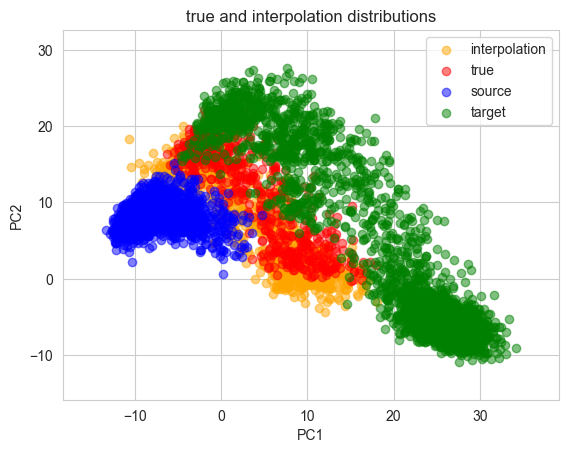
Interpolation:

Make interpolation distribution

For each of PCA and UMAP, interpolated and correct data can be compared. Also, source and target can be toggled on and off.

PCA ver.

scegot.plot_true_and_interpolation_distributions(
    interpolate_index=2,
    mode="pca",
    n_samples=1000,
    t=0.5,
    plot_source_and_target=True,
    alpha_true=0.5,
    # save=True,
    # save_path="./true_and_interpolation_distributions_pca.png"
)

UMAP ver.

scegot.plot_true_and_interpolation_distributions(
    interpolate_index=2,
    mode="umap",
    n_samples=500,
    t=0.5,
    plot_source_and_target=True,
    alpha_true=0.2,
    # save=True,
    # save_path="./true_and_interpolation_distributions_pca.png"
)

Transforming interpolated data with UMAP...

Interpolated animation of gene expression

PCA ver.

target_gene = "NKX1-2"
scegot.animate_gene_expression(
    target_gene,
    mode="pca",
    interpolate_interval=11,
    n_samples=5000,
    cmap="gnuplot2",
    # save=True,
    # save_path="./interpolate_video_pca.gif"
)

Interpolating between day0 and day0.5...

100%|██████████| 11/11 [00:00<00:00, 23.68it/s]

Interpolating between day0.5 and day1...

100%|██████████| 10/10 [00:00<00:00, 14.50it/s]

Interpolating between day1 and day1.5...

100%|██████████| 10/10 [00:01<00:00,  9.84it/s]

Interpolating between day1.5 and day2...

100%|██████████| 10/10 [00:01<00:00,  7.31it/s]

Creating animation...

Once Loop Reflect

UMAP ver.

Note that animation in umap space is time consuming due to the high computational cost of projecting into umap space.

%%time
target_gene = "NKX1-2"
scegot.animate_gene_expression(
    target_gene,
    mode="umap",
    interpolate_interval=11,
    n_samples=1000,
    cmap="gnuplot2",
    # save=True,
    # save_path="./interpolate_video_umap.gif"
)

Interpolating between day0 and day0.5...

100%|██████████| 11/11 [00:47<00:00,  4.31s/it]

Interpolating between day0.5 and day1...

100%|██████████| 10/10 [00:35<00:00,  3.55s/it]

Interpolating between day1 and day1.5...

100%|██████████| 10/10 [00:35<00:00,  3.56s/it]

Interpolating between day1.5 and day2...

100%|██████████| 10/10 [00:34<00:00,  3.45s/it]

Creating animation...

Once Loop Reflect

CPU times: user 3min 22s, sys: 22 s, total: 3min 44s
Wall time: 2min 34s

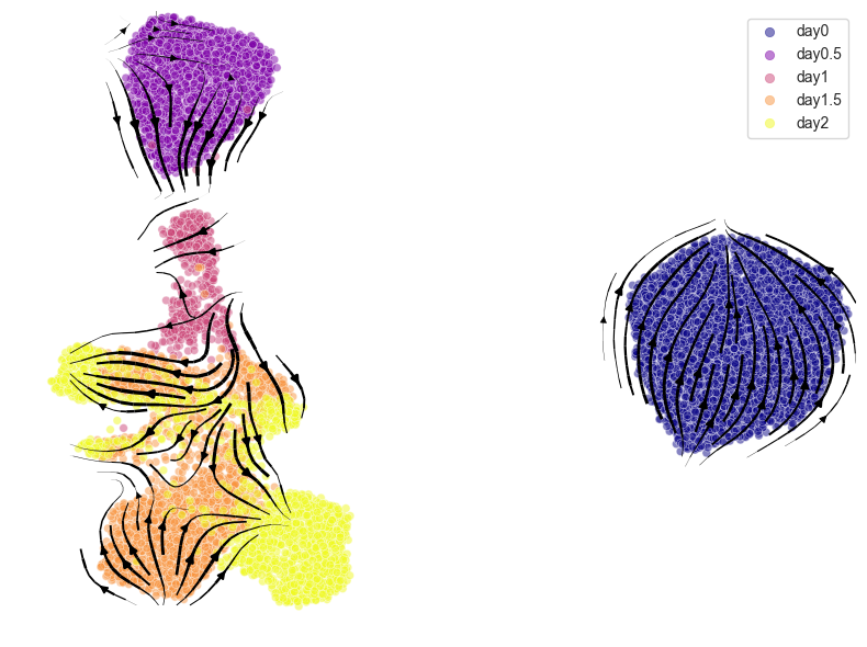
Cell velocity:

Plotting cell velocity

After the velocity is calculated using calculate_cell_velocities(), visualize it with plot_cell_velocity(). Both PCA and UMAP are supported.

PCA ver.

velocities = scegot.calculate_cell_velocities()
scegot.plot_cell_velocity(
    velocities,
    mode="pca",
    color_points="gmm",
    cluster_names=list(itertools.chain.from_iterable(cluster_names)),
    cmap="tab20",
    # save=True,
    # save_path="./cell_velocity_pca.png"
)

Calculating cell velocities between each day...

100%|██████████| 4/4 [00:00<00:00, 24.47it/s]

computing velocity graph (using 1/8 cores)

python(29403) MallocStackLogging: can't turn off malloc stack logging because it was not enabled.

    finished (0:00:02) --> added
    'velocity_graph', sparse matrix with cosine correlations (adata.uns)
computing velocity embedding
    finished (0:00:01) --> added
    'velocity_pca', embedded velocity vectors (adata.obsm)

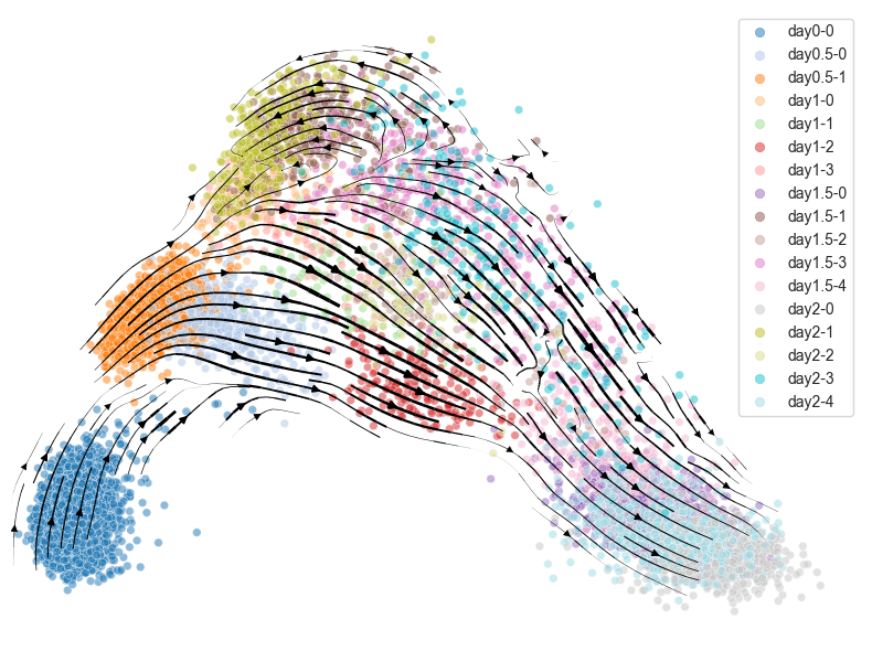
UMAP ver.

%%time
scegot.plot_cell_velocity(
    velocities,
    mode="umap",
    color_points="day",
    cmap="plasma",
    # save=True,
    # save_path="./cell_velocity_umap.png"
)

computing velocity graph (using 1/8 cores)

python(29564) MallocStackLogging: can't turn off malloc stack logging because it was not enabled.

    finished (0:00:01) --> added
    'velocity_graph', sparse matrix with cosine correlations (adata.uns)
computing velocity embedding
    finished (0:00:00) --> added
    'velocity_umap', embedded velocity vectors (adata.obsm)

CPU times: user 6.65 s, sys: 823 ms, total: 7.47 s
Wall time: 5.09 s

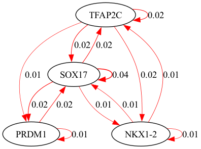
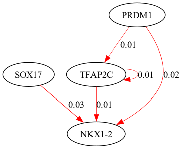
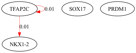
Gene regulatory network:

You can infer and visualize the Gene regulatory network between genes specified in selected_genes.

To display the network, you need to install GraphViz by referring to the following website.

https://www.graphviz.org/download/

%%time
GRNs, ridgeCVs = scegot.calculate_grns(
    selected_clusters=None,
    alpha_range=(-2, 2),
    cv=3,
    ridge_cv_fit_intercept=False,
    ridge_fit_intercept=False,
)

Calculating GRNs between each day...

100%|██████████| 4/4 [00:01<00:00,  3.63it/s]

CPU times: user 7.34 s, sys: 360 ms, total: 7.7 s
Wall time: 1.1 s

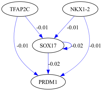
selected_genes = ["TFAP2C", "SOX17", "PRDM1", "NKX1-2"]
scegot.plot_grn_graph(
    GRNs,
    ridgeCVs,
    selected_genes,
    threshold=0.01,
    # save=True,
    # save_paths=[f"./grn_{day_name}.png" for day_name in DAY_NAMES],
    # save_format="png"
)

python(29628) MallocStackLogging: can't turn off malloc stack logging because it was not enabled.

alpha = 8.858667904100823

alpha = 37.92690190732246

python(29643) MallocStackLogging: can't turn off malloc stack logging because it was not enabled.

alpha = 37.92690190732246

python(29644) MallocStackLogging: can't turn off malloc stack logging because it was not enabled.

alpha = 100.0

python(29645) MallocStackLogging: can't turn off malloc stack logging because it was not enabled.

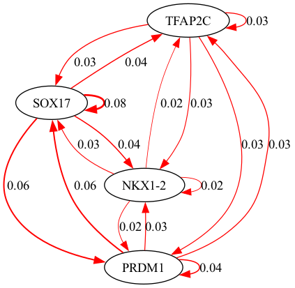
By passing an array of cluster names to selected_clusters, you can specify the clusters to be used in the GRN calculation.

%%time
selected_clusters = [[0, 0], [1, 1], [2, 0], [3, 1]] # [[data_point_index, cluster_number], ...]
GRNs_cluster, ridgeCVs_cluster = scegot.calculate_grns(
    selected_clusters=selected_clusters,
    alpha_range=(-2, 2),
    cv=3,
    ridge_cv_fit_intercept=False,
    ridge_fit_intercept=False,
)

Calculating GRNs between each day...

100%|██████████| 4/4 [00:00<00:00,  4.91it/s]

CPU times: user 5.57 s, sys: 483 ms, total: 6.05 s
Wall time: 819 ms

selected_genes = ["TFAP2C", "SOX17", "PRDM1", "NKX1-2"]
scegot.plot_grn_graph(
    GRNs_cluster,
    ridgeCVs_cluster,
    selected_genes,
    threshold=0.01,
    # save=True,
    # save_paths=[f"grn_selected_clusters_{day_name}" for day_name in DAY_NAMES],
    # save_format="png"
)

alpha = 8.858667904100823

python(29663) MallocStackLogging: can't turn off malloc stack logging because it was not enabled.

python(29665) MallocStackLogging: can't turn off malloc stack logging because it was not enabled.

alpha = 8.858667904100823

alpha = 2.06913808111479

python(29666) MallocStackLogging: can't turn off malloc stack logging because it was not enabled.

alpha = 8.858667904100823

python(29667) MallocStackLogging: can't turn off malloc stack logging because it was not enabled.

Reconstruction of the Waddington Landscape:

Both PCA and UMAP are supported.

%%time
Wpotential, F_all = scegot.calculate_waddington_potential(
    n_neighbors=100,
    knn_other_params={},
)

Calculating F between each day...

100%|██████████| 4/4 [00:00<00:00, 13.76it/s]

Applying knn ...
Computing kernel ...
CPU times: user 5.18 s, sys: 1.02 s, total: 6.2 s
Wall time: 2.84 s

Plot the Waddington potential in 3 dimensions. If gene_name is specified, the graph is colored by the expression level of the gene, and if gene_name is None, the graph is colored by the Waddington potential.

PCA ver.

import plotly.io as pio

scegot.plot_waddington_potential(
    Wpotential,
    mode="pca",
    gene_name=None,
    # save=True,
    # save_path="./waddington_potential_pca_potential.html"
)

Data type cannot be displayed: application/vnd.plotly.v1+json

gene_name = "NKX1-2"
scegot.plot_waddington_potential(
    Wpotential,
    mode="pca",
    gene_name=gene_name,
    # save=True,
    # save_path="./waddington_potential_pca_expression.html"
)

Data type cannot be displayed: application/vnd.plotly.v1+json

UMAP ver.

scegot.plot_waddington_potential(
    Wpotential,
    mode="umap",
    gene_name=None,
    # save=True,
    # save_path="./waddington_potential_umap_potential.html"
)

Data type cannot be displayed: application/vnd.plotly.v1+json

gene_name = "NKX1-2"
scegot.plot_waddington_potential(
    Wpotential,
    mode="umap",
    gene_name=gene_name,
    # save=True,
    # save_path="./waddington_potential_umap_expression.html"
)

Data type cannot be displayed: application/vnd.plotly.v1+json

You can also display a landscape instead of a plot of points.

PCA ver.

scegot.plot_waddington_potential_surface(
    Wpotential,
    mode="pca",
    # save=True,
    # save_path="./waddington_potential_surface_pca.html"
)

Data type cannot be displayed: application/vnd.plotly.v1+json

UMAP ver.

scegot.plot_waddington_potential_surface(
    Wpotential,
    mode="umap",
    # save=True,
    # save_path="./waddington_potential_surface_umap.html"
)

Data type cannot be displayed: application/vnd.plotly.v1+json